🚩 Using `redflag` with `sklearn`¶

As well as using redflag’s functions directly (see Basic_usage.ipynb), redflag has some sklearn transformers that you can use to detect possible issues in your data.

⚠️ Note that these transformers do not transform your data, they only raise warnings (red flags) if they find issues.

Let’s load some example data:

import pandas as pd

df = pd.read_csv('https://raw.githubusercontent.com/scienxlab/datasets/main/kgs/panoma-training-data.csv')

# Look at the transposed summary: each column in the DataFrame is a row here.
df.describe().T

	count	mean	std	min	25%	50%	75%	max
Depth	3966.0	882.674555	40.150056	784.402800	858.012000	888.339600	913.028400	963.320400
RelPos	3966.0	0.524999	0.286375	0.010000	0.282000	0.531000	0.773000	1.000000
Marine	3966.0	1.325013	0.589539	0.000000	1.000000	1.000000	2.000000	2.000000
GR	3966.0	64.367899	28.414603	12.036000	45.311250	64.840000	78.809750	200.000000
ILD	3966.0	5.240308	3.190416	0.340408	3.169567	4.305266	6.664234	32.136605
DeltaPHI	3966.0	3.469088	4.922310	-21.832000	1.000000	3.292500	6.124750	18.600000
PHIND	3966.0	13.008807	6.936391	0.550000	8.196250	11.781500	16.050000	52.369000
PE	3966.0	3.686427	0.815113	0.200000	3.123000	3.514500	4.241750	8.094000
Facies	3966.0	4.471004	2.406180	1.000000	2.000000	4.000000	6.000000	9.000000
LATITUDE	3966.0	37.632575	0.299398	37.180732	37.356426	37.500380	37.910583	38.063373
LONGITUDE	3966.0	-101.294895	0.230454	-101.646452	-101.389189	-101.325130	-101.106045	-100.987305
ILD_log10	3966.0	0.648860	0.251542	-0.468000	0.501000	0.634000	0.823750	1.507000
RHOB	3966.0	2288.861692	218.038459	1500.000000	2201.007475	2342.202051	2434.166399	2802.871147

Note that the features (e.g. GR, RHOB) are not independent records; they are correlated to themselves in depth.

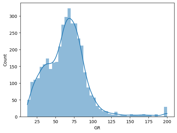
Furthermore, some of these features are clipped, e.g. the GR feature is clipped at a max value of 200:

import seaborn as sns

sns.histplot(df['GR'], lw=0, kde=True)

<Axes: xlabel='GR', ylabel='Count'>

../_images/9bf693b9868c28e3ef96bead37b8ce91cd2bfdea58fb7ed69ce8e6358f5c61a8.png

We will split this dataset by group (well name):

features = ['GR', 'RHOB', 'PE']

test_wells = ['CRAWFORD', 'STUART']

test_flag = df['Well Name'].isin(test_wells)

X_test = df.loc[test_flag, features]
y_test = df.loc[test_flag, 'Lithology']

X_train = df.loc[~test_flag, features]
y_train = df.loc[~test_flag, 'Lithology']

The `redflag` detector classes¶

There are two main kinds of object: detectors and comparators.

Detectors look for problems in your training and/or subsequent (e.g. validation, test, or production) data and are mostly unsupervised. There are several detectors:

ClipDetector() — looks for features that have been clipped.
CorrelationDetector() — looks for features that are correlated to themselves, which indicates that the data are likely not IID (in particular, not independent).
UnivariateOutlierDetector() — looks for outliers, considering each feature separately. Usually, you probably want to use OutlierDetector instead.
MultivariateOutlierDetector() — looks for outliers, considering all the features together. Usually, you probably want to use OutlierDetector instead.

The following detectors only run during training. In other words, they examine your data during model fitting, but do not look at data during subsequent calls to predict or score, etc.

ImportanceDetector() — looks at feature importance. Runs during fit only.
ImbalanceDetector() — looks for class imbalance in y. Runs during fit only. In other words, it can find class imbalance in the training data, but does not look at data during subsequent calls to predict or score, etc.

Finally, one detector is a bit different from the others because it runs in unsupervised mode on the training data, but in supervised mode on subsequent data. In other words, it can find outliers in the training data (based on some threshold), then it uses the statistics of the training data to decide what is an outlier in the subsequent data:

OutlierDetector() — looks for outliers. Runs during fit and transform.

Comparators are fully supervised. They learn things about your data during training, then look at subsequent (e.g. validation, test, or production) data and compare. They will not triger during model fitting, only during predict or score:

DistributionComparator() — checks that the distributions of the features are similar to those seen during training.
ImbalanceComparator()— checks that any class imbalance is similar to that seen during training. (Does not trigger if the training data is imbalanced; use ImbalanceDetector for that.) Note that this comparator does not work in ordinary sklearn.pipeline.Pipeline objects; use redflag.RfPipeline instead.

Using the ‘detector’ transformers¶

Let’s construct a pipeline from redflag’s transformers directly.

Let’s drop the clipped records of the GR log.

df = df.loc[df['GR'] < 200]

test_flag = df['Well Name'].isin(test_wells)

X_test = df.loc[test_flag, features]
y_test = df.loc[test_flag, 'Lithology']

X_train = df.loc[~test_flag, features]
y_train = df.loc[~test_flag, 'Lithology']

We know all this data is correlated to itself, so we can leave that check out.

We don’t think the class imbalance is too troubling, so we raise the threshold on that.

We’ll lower the confidence level of the outlier detector to 80% (i.e. we expect 20% of the data points will likely qualify as outliers). This might still trigger the detector in the training data.

Finally, we’ll lower the threshold for the distribution comparison. This is the minimum Wasserstein distance required to trigger the warning.

So here’s the new pipeline:

pipe = make_pipeline(StandardScaler(),
                     rf.ImbalanceDetector(threshold=0.5),
                     rf.ClipDetector(),
                     rf.OutlierDetector(p=0.80),
                     rf.DistributionComparator(threshold=0.25),
                     SVC())

Remember, feature 0 is no longer clipped, and the correlation detection is not being run. So we expect to see only the outlier issue, and the clipping issue with the RHOB column:

pipe.fit(X_train, y_train)

🚩 Feature 1 has samples that may be clipped.

🚩 There are more outliers than expected in the training data (839 vs 626).

Pipeline(steps=[('standardscaler', StandardScaler()),
                ('imbalancedetector', ImbalanceDetector(threshold=0.5)),
                ('clipdetector', ClipDetector()),
                ('outlierdetector',
                 OutlierDetector(p=0.8, threshold=2.154443705823081)),
                ('distributioncomparator',
                 DistributionComparator(threshold=0.25)),
                ('svc', SVC())])

In a Jupyter environment, please rerun this cell to show the HTML representation or trust the notebook.
On GitHub, the HTML representation is unable to render, please try loading this page with nbviewer.org.

The test dataset does not trigger the higher threshold for outliers. But with the new lower Wasserstein threshold, the distribution comparison fails for all of the features:

y_pred = pipe.predict(X_test)

🚩 Features 0, 1, 2 have distributions that are different from training.

The imbalance comparator¶

As mentioned, the ImbalanceComparator, is not compatible with ordinary Pipeline objects, because it requires y (class imbalance comparison only works on the target vector). An RfPipeline object is available to use with this comparator… but it will not work as part of another ordinary Pipeline (for the same reason: y will not be passed into it), so if you compose a multi-pipeline pipeline, make sure to use RfPipeline for all of it.

There is also a make_rf_pipeline() function that works just like make_pipeline, but it uses RfPipeline instead.

Let’s use it to check whether the imbalance in our test data is similar to the imbalance in the training data. When fitting a model, the comparator will never trigger:

pipe = rf.make_rf_pipeline(rf.ImbalanceComparator())

pipe.fit(X_train, y_train)

RfPipeline(steps=[('imbalancecomparator', ImbalanceComparator())])

But during transformation (therefore during prediction or other inference phases), it checks the imbalance is the same:

pipe.transform(X_test, y_test)

🚩 There is a different number of minority classes (2) compared to the training data (4).
🚩 The minority classes (sandstone, dolomite) are different from those in the training data (sandstone, dolomite, mudstone, wackestone).

array([[  66.276     , 2359.73324716,    3.591     ],
       [  77.252     , 2354.54679144,    3.341     ],
       [  82.899     , 2330.35783664,    3.064     ],
       ...,
       [  90.49      , 2193.06953439,    3.168     ],
       [  90.975     , 2192.32922081,    3.154     ],
       [  90.108     , 2176.62535394,    3.125     ]])

Making your own smoke detector¶

You can pass a detection function to a generic Detector, along with a warning to emit when it is triggered:

from redflag import Detector
import numpy as np

def has_nans(x) -> bool:
    """Returns True, i.e. triggers, if any samples are NaN."""
    return any(np.isnan(x))

negative_detector = Detector(has_nans, "are NaNs")

pipe = make_pipeline(negative_detector, SVC())
pipe.fit(X_train, y_train)

Pipeline(steps=[('detector',
                 Detector(func=<function BaseRedflagDetector.__init__.<locals>.<lambda> at 0x7fca2baef600>,
                          message='are NaNs')),
                ('svc', SVC())])

There are no NaNs.

You can use make_detector_pipeline to combine several tests into a single pipeline.

from redflag import make_detector_pipeline

def has_outliers(x):
    """Returns True, i.e. triggers, if any samples are negative."""
    return any(abs(x) > 5)

detectors = make_detector_pipeline([has_nans, has_outliers])

pipe = make_pipeline(StandardScaler(), detectors, SVC())
pipe.fit(X_train, y_train)

🚩 Features 0, 2 have samples that fail custom func has_outliers().

Pipeline(steps=[('standardscaler', StandardScaler()),
                ('pipeline',
                 Pipeline(steps=[('detector-1',
                                  Detector(func=<function BaseRedflagDetector.__init__.<locals>.<lambda> at 0x7fca2baef7e0>,
                                           message='fail custom func '
                                                   'has_nans()')),
                                 ('detector-2',
                                  Detector(func=<function BaseRedflagDetector.__init__.<locals>.<lambda> at 0x7fca2baef9c0>,
                                           message='fail custom func '
                                                   'has_outliers()'))])),
                ('svc', SVC())])

What to do about the warnings¶

If one of the detectors triggers, what should you do? Here are some ideas:

`ImbalanceDetector` and `ImbalanceComparator`¶

Check rf.class_counts(y) to see the support for each class in the dataset.
Check rf.minority_classes(y) to see which classes are considered ‘minority’.

This detector does not run during transform, only during fit. Usually, we don’t worry about imbalance in data we are predicting on. If this is a concern for you, you can use fit on it (and make a GitHub Issue about it, because we could add an option to run during transform as well).

`ClipDetector`¶

Make sure the clipping values seem reasonable and do not lose a lot of dynamic range in the data (e.g. don’t clip daily temperatures for Europe at 0 and 25 deg C).
Check that the clipped data cannot be dealt with in some other way (e.g. you can attenuate very large values with a log transformation, if it makes sense in your data).
Check that the clipped data should not simply be dropped from the dataset (e.g. if there are only a few values out of many, or if the other features also look suspicious for those records).

You may or may not be concerned about clipping. You may want to try training your models with and without the clipped records, to see if they make a difference to the model performance. I’m not aware of any research on this.

`CorrelationDetector`¶

If the data is correlated to shifted versions of itself, e.g. because the data points are contiguous in time or space (daily temperature records, spatial measurements of rock properties, etc), then the so-called IID assumption fails. In particular, your records are not independent. One of the big pitfalls with non-independent data is randomly splitting the data into train and test sets — you must not do this, it will result in information leakage and thus over-optimistic model evaulation. Instead, you should split the data using contiguous groups (date ranges, patient ID, borehole, or similar).

`OutlierDetector`¶

There are a lot of ways of looking for outliers in data. The outlier detector only implements one strategy:

Learn the robust location and covariance of the training data (you can think of these as outlier-insensitive, multi-dimensional analogs to mean and variance in a single random variable).
As with the Gaussian distribution, we expect a certain number of samples to fall far from the centre of this distribution. For example, we expect 99.7% of values to be within 3 standard deviations of the mean.
So, given a confidence level like 99.7%, redflag counts how many values are more than 3 SD’s away. If there are more than expected (e.g. we expect 3 samples out of 1000), the detector is triggered.
The default confidence level is 99% (you expect 1% of the data to be noise), but you can change it.

So the location and covariance are learned from the training data; the detector then runs on the training data and on future datasets during the prediction phase (test, val, and in production).

If the detector is triggered, you should check which samples are considered outliers with rf.get_outliers(method='mah', p=0.99) (without your value for p). This function returns the indices of the outlier samples. You can also use rf.expected_outliers(*X.shape, p=0.99) to check how many outliers you’d expect in the dataset, for a given value of p/.

You can check other methods, such as iso (isolation forest) to see if those also consider those samples to be outliers or not. If you think the samples are okay, you should keep them. If you think they are noise, you could remove them — but remember your model will not ‘know’ about these kinds of data points in the future and you should therefore remove them from future datasets too, before making predictions on them.

`DistributionComparator`¶

Here’s what this thing does:

When you call fit (e.g. during training), the detector learns the empirical, binned distributions of your features, one at a time. No warnings can be emitted during fitting, you are only learning the distributions.
When you call transform (e.g. during evaluation, testing, or in production), the detector compares the distributions in the data to those that were learned during fitting.
The comparison uses the 1-Wasserstein distance, or “earth mover’s distance”. Each feature is compared in turn; it is not a multivariate treatment. (If you’d like to see such a thing, please make a GitHub Issue, or have a crack at implementing it!)
If the distance is more than the threshold, 1 by default, the warning is triggered.

If this detector triggers, it’s a sign that you may have violated the ‘identical distribution’ part of the IID assumption. You should examine the distributions of the features in the training data vs the current data that triggered the detector. For example, you can do this visually with something like Seaborn’s displot or kdeplot functions.

A small difference, especially on just a few features, might just result from natural variance in the data and you may decide to ignore it. A large difference may be a result of forgetting to scale the data using the scaling parameters learned from the training data. A large difference could also result from trying to apply the model to a new ‘domain’, e.g. a new geographic location, set of patients, or type of widget.

If you’re in the model selection phase, it’s possible that a different train/test split will give more comparable distributions.

`ImportanceDetector`¶

This detector checks for both “too important” features and “not important enough” features, using thresholds you provide and some heuristics.

One or two very important features might indicate leakage: check that the features do not carry unintended information about the thing you are trying to predict. In particular, they should not carry information that will not be available to the model in production at prediction time. The classic example is trying to predict medical diagnosis using a patient number that contains encoded information about the patient’s diagnosis.

On the other hand, features with very low importance may not be useful to your model. If dimensionality is an issue, or the model is easily distracted by noise, you might improve performance by dropping one or more of these non-useful features. You will probably also improve the explainability of the model, which is often a desirable property.

🚩 Using redflag with sklearn¶

The redflag detector classes¶

Using the pre-built redflag pipeline¶

Using the ‘detector’ transformers¶

The imbalance comparator¶

Making your own smoke detector¶

What to do about the warnings¶

ImbalanceDetector and ImbalanceComparator¶

ClipDetector¶

CorrelationDetector¶

OutlierDetector¶

DistributionComparator¶

ImportanceDetector¶