Guess the colourmap from an image

The functions in unmap.unweave.py attempt to guess the colourmap from an image, using the graph implied by the colour co-occurrence matrix.

The following things will make things difficult:

• You don’t have a lot of pixels. Small images are hard to rip data from. We’d always like more pixels.

• The colourmap is not smooth. If there are strong colour contrasts in the colourmap, then the algorithm will struggle.

• The data distribution is not uniform. (It probably isn’t.) This wilkl tend to over-represent certain colours.

• There are a lot of annotations. Usually these get in the way of the data, especially if they use colours that also appear in the colourmap.

• The image is lossily compressed. Most PDFs contain JPEGs and JPEG is lossy. This means the colours are a bit garbled, especially around abrupt edges (like annotations!).

• The image has dithering. If the number of colours in the image has been reduced at some point, there’s a good chance it has been dithered.

• The image has hillshading or specularity. Cute 3D effects add another layer of complexity… but we can still have a go.

• The image is poor. If it’s a photo or scan of a paper document… well, now you ‘ve got the unknown transform from the data to the image, then the unknown transform of the image to the physical plot, then the unknown transform of the plot to the image you have. I mean, come on.

Finally, if you don’t have the colourmap information in a legend, then you may also not know the range of the data. There’s nothing you can do about that, unfortunately.

Things we may add in the future:

• Remove hillshade or specularity.

• Selectively remove certain colours. (Right now, colours that are different from anything else in the colourmap will likely be dropped anyway, e.g. black borders, because they are too far from the other colours.)

• Colourbar corrections for, e.g. a Gaussian distribution assumption.

• Match the language between unmap.py and unweave.py.

• Add a mask option so that a person can more easily just focus on the data area.

import unmap

unmap.__version__

'0.1.dev1+g175acc5'

Example

Let’s try to guess the colourmaps of some images on the web.

import numpy as np
from PIL import Image
import matplotlib.pyplot as plt
from urllib.request import urlretrieve
import ssl

ssl._create_default_https_context = ssl._create_unverified_context

def get_image_from_web(uri):
    f, _ = urlretrieve(uri)
    img = Image.open(f).convert('RGB')
    rgb_im = np.asarray(img)[..., :3] / 255.
    return rgb_im

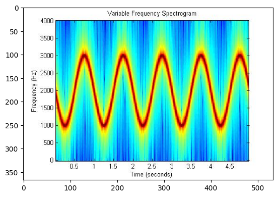
# Public domain image.
uri = 'https://upload.wikimedia.org/wikipedia/commons/2/2b/VariableFrequency.jpg'
img = get_image_from_web(uri)

plt.imshow(img)

<matplotlib.image.AxesImage at 0x7f2f2d27bca0>

We can give the image URI directly to guess_cmap(). It will read the image and try to construct a colourmap from it.

from unmap import guess_cmap_from_image

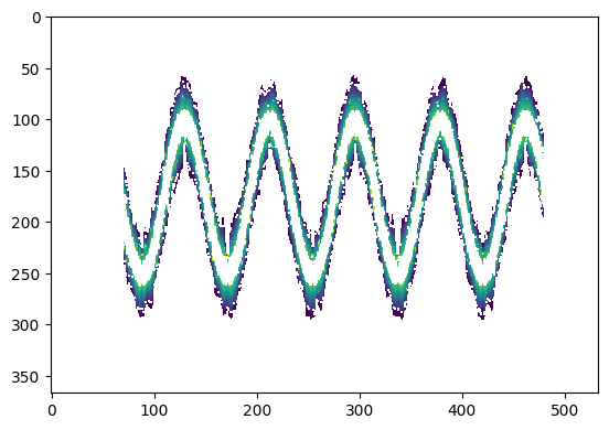
guess_cmap_from_image(uri)

recovered

under

bad

over

We got something, but it missed out the blues. We can try adjusting the maximum (Euclidean) distance allowed between neighbouring colours.

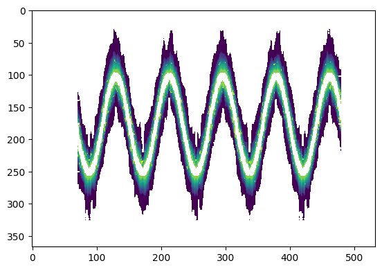
guess_cmap_from_image(uri, max_dist=0.4)

recovered

under

bad

over

We seem to be close; we’re getting a lot of blue-green though. The equilibrate option might help spread the colourbar out a bit more evenly.

guess_cmap_from_image(uri, max_dist=0.4, equilibrate=True)

recovered

under

bad

over

This helps a little, but sometimes this option can emphasize some abrupt colour boundaries, like the one in the red zone of the one above.

We could now give this colourmap to the unmapper:

from unmap import unmap

cmap = guess_cmap_from_image(uri, max_dist=0.4, equilibrate=True)
data = unmap(img, cmap=cmap)

Let’s look at the result:

import matplotlib.pyplot as plt

plt.imshow(data)

<matplotlib.image.AxesImage at 0x7f2f290bce80>

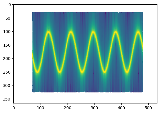
Too many colours were not mapped, because they are too far from anything in the colourmap. We can relax the threshold a bit:

data = unmap(img, cmap=cmap, threshold=0.4)
plt.imshow(data)

<matplotlib.image.AxesImage at 0x7f2f28b23040>

This result looks good.

Compare with the known colourmap

In this case, it looks like the actual colourmap is probably jet, let’s compare:

import matplotlib.cm as cm

cm.jet

jet

under

bad

over

This is comparable to the result we get when passing the known colourmap, jet:

data = unmap(img, cmap='jet', threshold=0.4)

plt.imshow(data)

<matplotlib.image.AxesImage at 0x7f2f28a214b0>

We don’t know the range of the data though, of course.

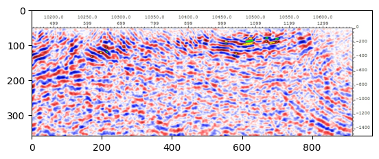
Try a seismic section

uri = "https://www.fathomgeophysics.com/images/post-image/post-image-seismic-data-analysis-972x360.jpg"

img = get_image_from_web(uri)

plt.imshow(img)

<matplotlib.image.AxesImage at 0x7f2f28a87b50>

guess_cmap_from_image(uri)

recovered

under

bad

over

Oh dear… seismic is tricky because the middle of thr distribution is so over-represented.

This time we need to tweak a few things: we need to allow more connections between colours (both min_weight and max_neighbours), and allow larger jumps in colour (max_dist).

guess_cmap_from_image(uri, min_weight=0.01, max_dist=0.15, max_neighbours=30)

recovered

under

bad

over